Control as a feedback system

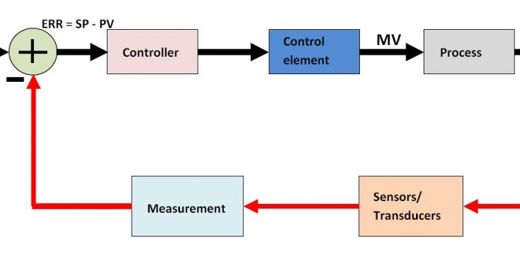
This is a basic feedback structure. Here, we are using the output value of the system to help us prepare the next output value. In this way, we can create systems that correct errors. Here we see a feedback loop with a value of one. We call this a unity feedback.

Here is a list of some relevant vocabulary, that will be used in the following sections:

Plant The term "Plant" is a carry-over term from chemical engineering to refer to the main system process. The plant is the preexisting system that does not (without the aid of a controller or a compensator) meet the given specifications. Plants are usually given "as is", and are not changeable. In the picture above, the plant is denoted with a P. Controller A controller, or a "compensator" is an additional system that is added to the plant to control the operation of the plant. The system can have multiple compensators, and they can appear anywhere in the system: Before the pick-off node, after the summer, before or after the plant, and in the feedback loop. In the picture above, our compensator is denoted with a C.

Some texts, or texts in other disciplines may refer to a "summer" as an adder.

Summer A summer is a symbol on a system diagram, (denoted above with parenthesis) that conceptually adds two or more input signals, and produces a single sum output signal. Pick-off node A pickoff node is simply a fancy term for a split in a wire. Forward Path The forward path in the feedback loop is the path after the summer, that travels through the plant and towards the system output. Reverse Path The reverse path is the path after the pick-off node, that loops back to the beginning of the system. This is also known as the "feedback path". Unity feedback When the multiplicative value of the feedback path is 1.

Negative vs Positive Feedback[edit]

It turns out that negative feedback is almost always the most useful type of feedback. When we subtract the value of the output from the value of the input (our desired value), we get a value called the error signal. The error signal shows us how far off our output is from our desired input.

Positive feedback has the property that signals tend to reinforce themselves, and grow larger. In a positive feedback system, noise from the system is added back to the input, and that in turn produces more noise. As an example of a positive feedback system, consider an audio amplification system with a speaker and a microphone. Placing the microphone near the speaker creates a positive feedback loop, and the result is a sound that grows louder and louder. Because the majority of noise in an electrical system is high-frequency, the sound output of the system becomes high-pitched.

Example: State-Space Equation[edit]

In the previous chapter, we showed you this picture:

Now, we will derive the I/O relationship into the state-space equations. If we examine the inner-most feedback loop, we can see that the forward path has an integrator system, 1s{\displaystyle {\frac {1}{s}}}, and the feedback loop has the matrix value A. If we take the transfer function only of this loop, we get:

Tinner(s)=1s1−1sA=1s−A{\displaystyle T_{inner}(s)={\frac {\frac {1}{s}}{1-{\frac {1}{s}}A}}={\frac {1}{s-A}}}

Pre-multiplying by the factor B, and post-multiplying by C, we get the transfer function of the entire lower-half of the loop:

Tlower(s)=B(1s−A)C{\displaystyle T_{lower}(s)=B\left({\frac {1}{s-A}}\right)C}

We can see that the upper path (D) and the lower-path Tlower are added together to produce the final result:

Ttotal(s)=B(1s−A)C+D{\displaystyle T_{total}(s)=B\left({\frac {1}{s-A}}\right)C+D}

Now, for an alternate method, we can assume that x' is the value of the inner-feedback loop, right before the integrator. This makes sense, since the integral of x' should be x (which we see from the diagram that it is. Solving for x', with an input of u, we get:

x′=Ax+Bu{\displaystyle x'=Ax+Bu}

This is because the value coming from the feedback branch is equal to the value x times the feedback loop matrix A, and the value coming from the left of the sumer is the input u times the matrix B.

If we keep things in terms of x and u, we can see that the system output is the sum of u times the feed-forward value D, and the value of x times the value C:

y=Cx+Du{\displaystyle y=Cx+Du}

These last two equations are precisely the state-space equations of our system.

Feedback Loop Transfer Function[edit]

We can solve for the output of the system by using a series of equations:

E(s)=X(s)−Y(s){\displaystyle E(s)=X(s)-Y(s)} Y(s)=G(s)E(s){\displaystyle Y(s)=G(s)E(s)}

and when we solve for Y(s) we get:

[Feedback Transfer Function]

Y(s)=X(s)Gp(s)1+Gp(s){\displaystyle Y(s)=X(s){\frac {Gp(s)}{1+Gp(s)}}}

The reader is encouraged to use the above equations to derive the result by themselves.

The function E(s) is known as the error signal. The error signal is the difference between the system output (Y(s)), and the system input (X(s)). Notice that the error signal is now the direct input to the system G(s). X(s) is now called the reference input. The purpose of the negative feedback loop is to make the system output equal to the system input, by identifying large differences between X(s) and Y(s) and correcting for them.

Example: Elevator[edit]

Here is a simple example of reference inputs and feedback systems:

There is an elevator in a certain building with 5 floors. Pressing button "1" will take you to the first floor, and pressing button "5" will take you to the fifth floor, etc. For reasons of simplicity, only one button can be pressed at a time.

Pressing a particular button is the reference input of the system. Pressing "1" gives the system a reference input of 1, pressing "2" gives the system a reference input of 2, etc. The elevator system then, tries to make the output (the physical floor location of the elevator) match the reference input (the button pressed in the elevator). The error signal, e(t), represents the difference between the reference input x(t), and the physical location of the elevator at time t, y(t).

Let's say that the elevator is on the first floor, and the button "5" is pressed at time t0. The reference input then becomes a step function:

x(t)=5u(t−t0){\displaystyle x(t)=5u(t-t_{0})}

Where we are measuring in units of "floors". At time t0, the error signal is:

e(t0)=x(t0)−y(t0)=5−1=4{\displaystyle e(t_{0})=x(t_{0})-y(t_{0})=5-1=4}

Which means that the elevator needs to travel upwards 4 more floors. At time t1, when the elevator is at the second floor, the error signal is:

e(t1)=x(t1)−y(t1)=5−2=3{\displaystyle e(t_{1})=x(t_{1})-y(t_{1})=5-2=3}

Which means the elevator has 3 more floors to go. Finally, at time t4, when the elevator reaches the top, the error signal is:

e(t4)=x(t4)−y(t4)=5−5=0{\displaystyle e(t_{4})=x(t_{4})-y(t_{4})=5-5=0}

And when the error signal is zero, the elevator stops moving. In essence, we can define three cases:

• e(t) is positive: In this case, the elevator goes up one floor, and checks again.
• e(t) is zero: The elevator stops.
• e(t) is negative: The elevator goes down one floor, and checks again.